Machine Learning Exercises In Python, Part 2
24th January 2015This post is part of a series covering the exercises from Andrew Ng's machine learning class on Coursera. The original code, exercise text, and data files for this post are available here.
Part 1 - Simple Linear Regression
Part 2 - Multivariate Linear Regression
Part 3 - Logistic Regression
Part 4 - Multivariate Logistic Regression
Part 5 - Neural Networks
Part 6 - Support Vector Machines
Part 7 - K-Means Clustering & PCA
Part 8 - Anomaly Detection & Recommendation
In part 1 of my series on machine learning in Python, we covered the first part of exercise 1 in Andrew Ng's Machine Learning class. In this post we'll wrap up exercise 1 by completing part 2 of the exercise. If you recall, in part 1 we implemented linear regression to predict the profits of a new food truck based on the population of the city that the truck would be placed in. For part 2 we've got a new task - predict the price that a house will sell for. The difference this time around is we have more than one dependent variable. We're given both the size of the house in square feet, and the number of bedrooms in the house. Can we easily extend our previous code to handle multiple linear regression? Let's find out!
First let's take a look at the data.
path = os.getcwd() + '\data\ex1data2.txt'
data2 = pd.read_csv(path, header=None, names=['Size', 'Bedrooms', 'Price'])
data2.head()
| Size | Bedrooms | Price | |
|---|---|---|---|
| 0 | 2104 | 3 | 399900 |
| 1 | 1600 | 3 | 329900 |
| 2 | 2400 | 3 | 369000 |
| 3 | 1416 | 2 | 232000 |
| 4 | 3000 | 4 | 539900 |
Notice that the scale of the values for each variable is vastly different. A house will typically have 2-5 bedrooms but may have anywhere from hundreds to thousands of square feet. If we were to run our regression algorithm on this data as-is, the "size" variable would be weighted too heavily and would end up dwarfing any contributions from the "number of bedrooms" feature. To fix this, we need to do something called "feature normalization". That is, we need to adjust the scale of the features to level the playing field. One way to do this is by subtracting from each value in a feature the mean of that feature, and then dividing by the standard deviation. Fortunately this is one line of code using pandas.
data2 = (data2 - data2.mean()) / data2.std()
data2.head()
| Size | Bedrooms | Price | |
|---|---|---|---|
| 0 | 0.130010 | -0.223675 | 0.475747 |
| 1 | -0.504190 | -0.223675 | -0.084074 |
| 2 | 0.502476 | -0.223675 | 0.228626 |
| 3 | -0.735723 | -1.537767 | -0.867025 |
| 4 | 1.257476 | 1.090417 | 1.595389 |
Next, we need to modify our implementation of linear regression from part 1 to handle more than 1 dependent variable. Or do we? Let's take a look at the code for the gradient descent function again.
def gradientDescent(X, y, theta, alpha, iters):
    temp = np.matrix(np.zeros(theta.shape))
    parameters = int(theta.ravel().shape[1])
    cost = np.zeros(iters)

    for i in range(iters):
        error = (X * theta.T) - y

        for j in range(parameters):
            term = np.multiply(error, X[:,j])
            temp[0,j] = theta[0,j] - ((alpha / len(X)) * np.sum(term))

        theta = temp
        cost[i] = computeCost(X, y, theta)

    return theta, cost
Look closely at the line of code calculating the error term: error = (X * theta.T) - y. It might not be obvious at first but we're using all matrix operations! This is the power of linear algebra at work. This code will work correctly no matter how many variables (columns) are in X, as long as the number of parameters in theta agree. Similarly, it will compute the error term for every row in X as long as the number of rows in y agree. On top of that, it's a very efficient calculation. This is a powerful way to apply ANY expression to a large number of instances at once.
Since both our gradient descent and cost function are using matrix operations, there is in fact no change to the code necessary to handle multiple linear regression. Let's test it out. We first need to perform a few initializations to create the appropriate matrices to pass to our functions.
# add ones column
data2.insert(0, 'Ones', 1)

# set X (training data) and y (target variable)
cols = data2.shape[1]
X2 = data2.iloc[:,0:cols-1]
y2 = data2.iloc[:,cols-1:cols]

# convert to matrices and initialize theta
X2 = np.matrix(X2.values)
y2 = np.matrix(y2.values)
theta2 = np.matrix(np.array([0,0,0]))
Now we're ready to give it a try. Let's see what happens.
# perform linear regression on the data set
g2, cost2 = gradientDescent(X2, y2, theta2, alpha, iters)

# get the cost (error) of the model
computeCost(X2, y2, g2)
0.13070336960771897
Looks promising! We can also plot the training progress to confirm that the error was in fact decreasing with each iteration of gradient descent.
fig, ax = plt.subplots(figsize=(12,8))
ax.plot(np.arange(iters), cost2, 'r')
ax.set_xlabel('Iterations')
ax.set_ylabel('Cost')
ax.set_title('Error vs. Training Epoch')
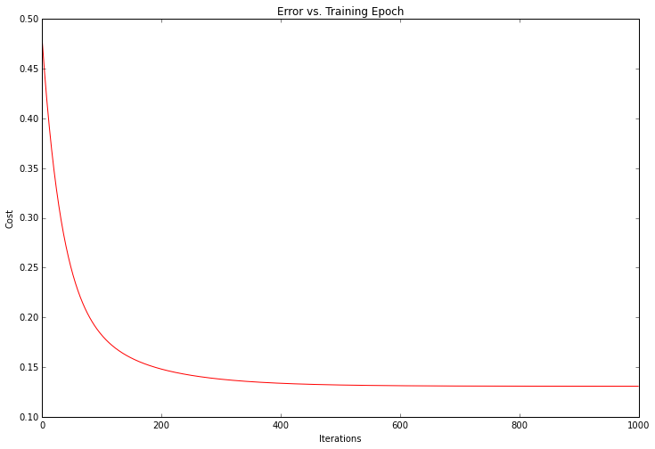
The cost, or error of the solution, dropped with each sucessive iteration until it bottomed out. This is exactly what we would expect to happen. It looks like our algorithm worked.
It's worth noting that we don't HAVE to implement any algorithms from scratch to solve this problem. The great thing about Python is its huge developer community and abundance of open-source software. In the machine learning realm, the top Python library is scikit-learn. Let's see how we could have handled our simple linear regression task from part 1 using scikit-learn's linear regression class.
from sklearn import linear_model
model = linear_model.LinearRegression()
model.fit(X, y)
It doesn't get much easier than that. There are lots of parameters to the "fit" method that we could have tweaked depending on how we want the algorithm to function, but the defaults are sensible enough for our problem that I left them alone. Let's try plotting the fitted parameters to see how it compares to our earlier results.
x = np.array(X[:, 1].A1)
f = model.predict(X).flatten()

fig, ax = plt.subplots(figsize=(12,8))
ax.plot(x, f, 'r', label='Prediction')
ax.scatter(data.Population, data.Profit, label='Traning Data')
ax.legend(loc=2)
ax.set_xlabel('Population')
ax.set_ylabel('Profit')
ax.set_title('Predicted Profit vs. Population Size')
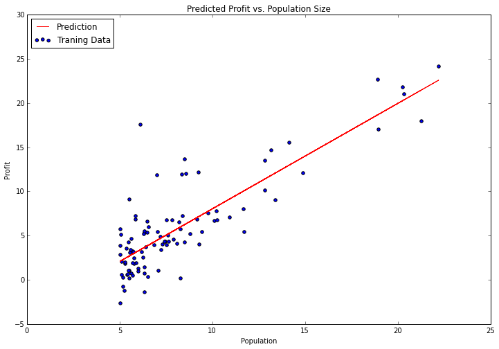
Notice I'm using the "predict" function to get the predicted y values in order to draw the line. This is much easier than trying to do it manually. Scikit-learn has a great API with lots of convenience functions for typical machine learning workflows. We'll explore some of these in more detail in future posts.
That's it for today. In part 3, we'll take a look at exercise 2 and dive into some classification tasks using logistic regression.