Machine Learning Exercises In Python, Part 3

This post is part of a series covering the exercises from Andrew Ng's machine learning class on Coursera. The original code, exercise text, and data files for this post are available here.

Part 1 - Simple Linear Regression
Part 2 - Multivariate Linear Regression
Part 3 - Logistic Regression
Part 4 - Multivariate Logistic Regression
Part 5 - Neural Networks
Part 6 - Support Vector Machines
Part 7 - K-Means Clustering & PCA
Part 8 - Anomaly Detection & Recommendation

In part 2 of the series we wrapped up our implementation of multivariate linear regression using gradient descent and applied it to a simple housing prices data set. In this post we’re going to switch our objective from predicting a continuous value (regression) to classifying a result into two or more discrete buckets (classification) and apply it to a student admissions problem. Suppose that you are the administrator of a university department and you want to determine each applicant's chance of admission based on their results on two exams. You have historical data from previous applicants that you can use as a training set. For each training example, you have the applicant's scores on two exams and the admissions decision. To accomplish this, we're going to build a classification model that estimates the probability of admission based on the exam scores using a somewhat confusingly-named technique called logistic regression.

Logistic Regression

You may be wondering – why are we using a “regression” algorithm on a classification problem? Although the name seems to indicate otherwise, logistic regression is actually a classification algorithm. I suspect it’s named as such because it’s very similar to linear regression in its learning approach, but the cost and gradient functions are formulated differently. In particular, logistic regression uses a sigmoid or “logit” activation function instead of the continuous output in linear regression (hence the name). We’ll see more later on when we dive into the implementation.

To get started, let’s import and examine the data set we’ll be working with.

import numpy as np
import pandas as pd
import matplotlib.pyplot as plt
%matplotlib inline

import os
path = os.getcwd() + '\data\ex2data1.txt'
data = pd.read_csv(path, header=None, names=['Exam 1', 'Exam 2', 'Admitted'])
data.head()

	Exam 1	Exam 2	Admitted
0	34.623660	78.024693	0
1	30.286711	43.894998	0
2	35.847409	72.902198	0
3	60.182599	86.308552	1
4	79.032736	75.344376	1

There are two continuous independent variables in the data - “Exam 1” and “Exam 2”. Our prediction target is the “Admitted” label, which is binary-valued. A value of 1 means the student was admitted and a value of 0 means the student was not admitted. Let’s see this graphically with a scatter plot of the two scores and use color coding to visualize if the example is positive or negative.

positive = data[data['Admitted'].isin([1])]
negative = data[data['Admitted'].isin([0])]

fig, ax = plt.subplots(figsize=(12,8))
ax.scatter(positive['Exam 1'], positive['Exam 2'], s=50, c='b', marker='o', label='Admitted')
ax.scatter(negative['Exam 1'], negative['Exam 2'], s=50, c='r', marker='x', label='Not Admitted')
ax.legend()
ax.set_xlabel('Exam 1 Score')
ax.set_ylabel('Exam 2 Score')

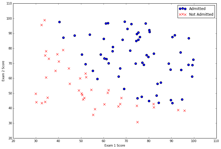
From this plot we can see that there’s a nearly linear decision boundary. It curves a bit so we can’t classify all of the examples correctly using a straight line, but we should be able to get pretty close. Now we need to implement logistic regression so we can train a model to find the optimal decision boundary and make class predictions. The first step is to implement the sigmoid function.

def sigmoid(z):
    return 1 / (1 + np.exp(-z))

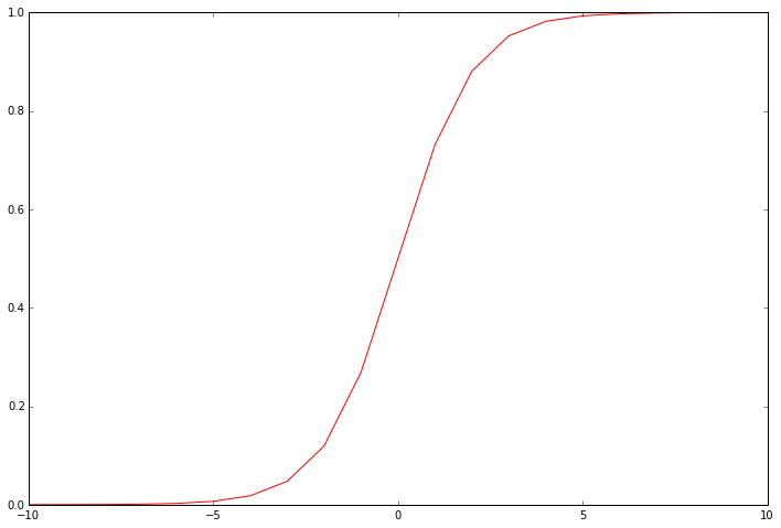
This function is the “activation” function for the output of logistic regression. It converts a continuous input into a value between zero and one. This value can be interpreted as the class probability, or the likelihood that the input example should be classified positively. Using this probability along with a threshold value, we can obtain a discrete label prediction. It helps to visualize the function’s output to see what it’s really doing.

nums = np.arange(-10, 10, step=1)

fig, ax = plt.subplots(figsize=(12,8))
ax.plot(nums, sigmoid(nums), 'r')

Our next step is to write the cost function. Remember that the cost function evaluates the performance of the model on the training data given a set of model parameters. Here’s the cost function for logistic regression.

def cost(theta, X, y):
    theta = np.matrix(theta)
    X = np.matrix(X)
    y = np.matrix(y)
    first = np.multiply(-y, np.log(sigmoid(X * theta.T)))
    second = np.multiply((1 - y), np.log(1 - sigmoid(X * theta.T)))
    return np.sum(first - second) / (len(X))

Note that we reduce the output down to a single scalar value, which is the sum of the “error” quantified as a function of the difference between the class probability assigned by the model and the true label of the example. The implementation is completely vectorized – it’s computing the model’s predictions for the whole data set in one statement (sigmoid(X * theta.T)). If the math here isn’t making sense, refer to the exercise text I linked to above for a more detailed explanation.

We can test the cost function to make sure it’s working, but first we need to do some setup.

# add a ones column - this makes the matrix multiplication work out easier
data.insert(0, 'Ones', 1)

# set X (training data) and y (target variable)
cols = data.shape[1]
X = data.iloc[:,0:cols-1]
y = data.iloc[:,cols-1:cols]

# convert to numpy arrays and initalize the parameter array theta
X = np.array(X.values)
y = np.array(y.values)
theta = np.zeros(3)

I like to check the shape of the data structures I’m working with fairly often to convince myself that their values are sensible. This technique if very useful when implementing matrix multiplication.

X.shape, theta.shape, y.shape

((100L, 3L), (3L,), (100L, 1L))

Now let’s compute the cost for our initial solution given zeros for the model parameters, here represented as “theta”.

cost(theta, X, y)

0.69314718055994529

Now that we have a working cost function, the next step is to write a function that computes the gradient of the model parameters to figure out how to change the parameters to improve the outcome of the model on the training data. Recall that with gradient descent we don’t just randomly jigger around the parameter values and see what works best. At each training iteration we update the parameters in a way that’s guaranteed to move them in a direction that reduces the training error (i.e. the “cost”). We can do this because the cost function is differentiable. The calculus involved in deriving the equation is well beyond the scope of this blog post, but the full equation is in the exercise text. Here’s the function.

def gradient(theta, X, y):
    theta = np.matrix(theta)
    X = np.matrix(X)
    y = np.matrix(y)
    
    parameters = int(theta.ravel().shape[1])
    grad = np.zeros(parameters)
    
    error = sigmoid(X * theta.T) - y
    
    for i in range(parameters):
        term = np.multiply(error, X[:,i])
        grad[i] = np.sum(term) / len(X)
    
    return grad

Note that we don't actually perform gradient descent in this function - we just compute a single gradient step. In the exercise, an Octave function called "fminunc" is used to optimize the parameters given functions to compute the cost and the gradients. Since we're using Python, we can use SciPy's optimization API to do the same thing.

import scipy.optimize as opt
result = opt.fmin_tnc(func=cost, x0=theta, fprime=gradient, args=(X, y))
cost(result[0], X, y)

0.20357134412164668

We now have the optimal model parameters for our data set. Next we need to write a function that will output predictions for a dataset X using our learned parameters theta. We can then use this function to score the training accuracy of our classifier.

def predict(theta, X):
    probability = sigmoid(X * theta.T)
    return [1 if x >= 0.5 else 0 for x in probability]

theta_min = np.matrix(result[0])
predictions = predict(theta_min, X)
correct = [1 if ((a == 1 and b == 1) or (a == 0 and b == 0)) else 0 for (a, b) in zip(predictions, y)]
accuracy = (sum(map(int, correct)) % len(correct))
print 'accuracy = {0}%'.format(accuracy)

accuracy = 89%

Our logistic regression classifer correctly predicted if a student was admitted or not 89% of the time. Not bad! Keep in mind that this is training set accuracy though. We didn't keep a hold-out set or use cross-validation to get a true approximation of the accuracy so this number is likely higher than its true performance (this topic is covered in a later exercise).

Regularized Logistic Regression

Now that we have a working implementation of logistic regression, we'll going to improve the algorithm by adding regularization. Regularization is a term in the cost function that causes the algorithm to prefer "simpler" models (in this case, models will smaller coefficients). The theory is that this helps to minimize overfitting and improve the model's ability to generalize. We’ll apply our regularized version of logistic regression to a slightly more challenging problem. Suppose you are the product manager of the factory and you have the test results for some microchips on two different tests. From these two tests, you would like to determine whether the microchips should be accepted or rejected. To help you make the decision, you have a data set of test results on past microchips, from which you can build a logistic regression model.

Let's start by visualizing the data.

path = os.getcwd() + '\data\ex2data2.txt'
data2 = pd.read_csv(path, header=None, names=['Test 1', 'Test 2', 'Accepted'])

positive = data2[data2['Accepted'].isin([1])]
negative = data2[data2['Accepted'].isin([0])]

fig, ax = plt.subplots(figsize=(12,8))
ax.scatter(positive['Test 1'], positive['Test 2'], s=50, c='b', marker='o', label='Accepted')
ax.scatter(negative['Test 1'], negative['Test 2'], s=50, c='r', marker='x', label='Rejected')
ax.legend()
ax.set_xlabel('Test 1 Score')
ax.set_ylabel('Test 2 Score')

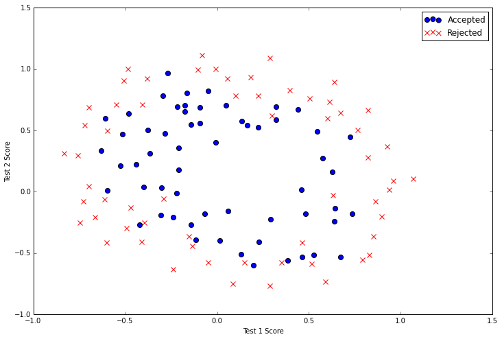
This data looks a bit more complicated than the previous example. In particular, you'll notice that there is no linear decision boundary that will perform well on this data. One way to deal with this using a linear technique like logistic regression is to construct features that are derived from polynomials of the original features. We can try creating a bunch of polynomial features to feed into the classifier.

degree = 5
x1 = data2['Test 1']
x2 = data2['Test 2']

data2.insert(3, 'Ones', 1)

for i in range(1, degree):
    for j in range(0, i):
        data2['F' + str(i) + str(j)] = np.power(x1, i-j) * np.power(x2, j)

data2.drop('Test 1', axis=1, inplace=True)
data2.drop('Test 2', axis=1, inplace=True)

data2.head()

	Accepted	Ones	F10	F20	F21	F30	F31	F32
0	1	1	0.051267	0.002628	0.035864	0.000135	0.001839	0.025089
1	1	1	-0.092742	0.008601	-0.063523	-0.000798	0.005891	-0.043509
2	1	1	-0.213710	0.045672	-0.147941	-0.009761	0.031616	-0.102412
3	1	1	-0.375000	0.140625	-0.188321	-0.052734	0.070620	-0.094573
4	1	1	-0.513250	0.263426	-0.238990	-0.135203	0.122661	-0.111283

Now we need to modify the cost and gradient functions to include the regularization term. In each case, the regularizer is added on to the previous calculation. Here’s the updated cost function.

def costReg(theta, X, y, learningRate):
    theta = np.matrix(theta)
    X = np.matrix(X)
    y = np.matrix(y)
    first = np.multiply(-y, np.log(sigmoid(X * theta.T)))
    second = np.multiply((1 - y), np.log(1 - sigmoid(X * theta.T)))
    reg = (learningRate / 2 * len(X)) * np.sum(np.power(theta[:,1:theta.shape[1]], 2))
    return np.sum(first - second) / (len(X)) + reg

Notice that we’ve added a new variable called “reg” that is a function of the parameter values. As the parameters get larger, the penalization added to the cost function increases. Also note that we’ve added a new “learning rate” parameter to the function. This is also part of the regularization term in the equation. The learning rate gives us a new hyper-parameter that we can use to tune how much weight the regularization holds in the cost function.

Next we’ll add regularization to the gradient function.

def gradientReg(theta, X, y, learningRate):
    theta = np.matrix(theta)
    X = np.matrix(X)
    y = np.matrix(y)
    
    parameters = int(theta.ravel().shape[1])
    grad = np.zeros(parameters)
    
    error = sigmoid(X * theta.T) - y
    
    for i in range(parameters):
        term = np.multiply(error, X[:,i])
        
        if (i == 0):
            grad[i] = np.sum(term) / len(X)
        else:
            grad[i] = (np.sum(term) / len(X)) + ((learningRate / len(X)) * theta[:,i])
    
    return grad

Just as with the cost function, the regularization term is added on to the original calculation. However, unlike the cost function, we included logic to make sure that the first parameter is not regularized. The intuition behind this decision is that the first parameter is considered the “bias” or “intercept” of the model and shouldn’t be penalized.

We can test out the new functions just as we did before.

# set X and y (remember from above that we moved the label to column 0)
cols = data2.shape[1]
X2 = data2.iloc[:,1:cols]
y2 = data2.iloc[:,0:1]

# convert to numpy arrays and initalize the parameter array theta
X2 = np.array(X2.values)
y2 = np.array(y2.values)
theta2 = np.zeros(11)

learningRate = 1

costReg(theta2, X2, y2, learningRate)

0.6931471805599454

We can also re-use the optimization code from earlier to find the optimal model parameters.

result2 = opt.fmin_tnc(func=costReg, x0=theta2, fprime=gradientReg, args=(X2, y2, learningRate))
result2

(array([ 0.35872309, -3.22200653, 18.97106363, -4.25297831,
18.23053189, 20.36386672, 8.94114455, -43.77439015,
-17.93440473, -50.75071857, -2.84162964]), 110, 1)

Finally, we can use the same method we applied earlier to create label predictions for the training data and evaluate the performance of the model.

theta_min = np.matrix(result2[0])
predictions = predict(theta_min, X2)
correct = [1 if ((a == 1 and b == 1) or (a == 0 and b == 0)) else 0 for (a, b) in zip(predictions, y2)]
accuracy = (sum(map(int, correct)) % len(correct))
print 'accuracy = {0}%'.format(accuracy)

accuracy = 91%

That's all for part 3! In the next post in the series we'll expand on our implementation of logistic regression to tackle multi-class image classification.