Machine Learning Exercises In Python, Part 4

This post is part of a series covering the exercises from Andrew Ng's machine learning class on Coursera. The original code, exercise text, and data files for this post are available here.

Part 1 - Simple Linear Regression
Part 2 - Multivariate Linear Regression
Part 3 - Logistic Regression
Part 4 - Multivariate Logistic Regression
Part 5 - Neural Networks
Part 6 - Support Vector Machines
Part 7 - K-Means Clustering & PCA
Part 8 - Anomaly Detection & Recommendation

In part three of this series we implemented both simple and regularized logistic regression, completing our Python implementation of the second exercise from Andrew Ng's machine learning class. There's a limitation with our solution though - it only works for binary classification. In this post we'll extend our solution from the previous exercise to handle multi-class classification. In doing so, we'll cover the first half of exercise 3 and set ourselves up for the next big topic, neural networks.

Just a quick note on syntax - to show the output of a statement I'm appending the result in the code block with a ">" to indicate that it's the result of running the previous statement. If the result is very long (more than 1-2 lines) then I'm sticking it below the code block in a separate block of its own. Hopefully it's clear which statements are input and which are output.

Our task in this exercise is to use logistic regression to recognize hand-written digits (0 to 9). Let's get started by loading the data set. Unlike the previous examples, our data file is in a format native to MATLAB and not automatically recognizable by pandas, so to load it in Python we need to use a SciPy utility (remember the data files are available at the link at the top of the post).

import numpy as np
import pandas as pd
import matplotlib.pyplot as plt
from scipy.io import loadmat
%matplotlib inline

data = loadmat('data/ex3data1.mat')
data

{'X': array([[ 0.,  0.,  0., ...,  0.,  0.,  0.],
        [ 0.,  0.,  0., ...,  0.,  0.,  0.],
        [ 0.,  0.,  0., ...,  0.,  0.,  0.],
        ..., 
        [ 0.,  0.,  0., ...,  0.,  0.,  0.],
        [ 0.,  0.,  0., ...,  0.,  0.,  0.],
        [ 0.,  0.,  0., ...,  0.,  0.,  0.]]),
 '__globals__': [],
 '__header__': 'MATLAB 5.0 MAT-file, Platform: GLNXA64, Created on: Sun Oct 16 13:09:09 2011',
 '__version__': '1.0',
 'y': array([[10],
        [10],
        [10],
        ..., 
        [ 9],
        [ 9],
        [ 9]], dtype=uint8)}

Let's quickly examine the shape of the arrays we just loaded into memory.

data['X'].shape, data['y'].shape

> ((5000L, 400L), (5000L, 1L))

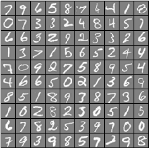
Great, we've got our data loaded. The images are represented in martix X as a 400-dimensional vector (of which there are 5,000 of them). The 400 "features" are grayscale intensities of each pixel in the original 20 x 20 image. The class labels are in the vector y as a numeric class representing the digit that's in the image. There's an illustration below gives an example of what some of the digits look like. Each grey box with a white hand-drawn digit represents on 400-dimensional row in our dataset.

Our first task is to modify our logistic regression implementation to be completely vectorized (i.e. no "for" loops). This is because vectorized code, in addition to being short and concise, is able to take advantage of linear algebra optimizations and is typically much faster than iterative code. However if you look at our cost function implementation from exercise 2, it's already vectorized! So we can re-use the same implementation here. Note we're skipping straight to the final, regularized version.

def sigmoid(z):
    return 1 / (1 + np.exp(-z))

def cost(theta, X, y, learningRate):
    theta = np.matrix(theta)
    X = np.matrix(X)
    y = np.matrix(y)
    first = np.multiply(-y, np.log(sigmoid(X * theta.T)))
    second = np.multiply((1 - y), np.log(1 - sigmoid(X * theta.T)))
    reg = (learningRate / 2 * len(X)) * np.sum(np.power(theta[:,1:theta.shape[1]], 2))
    return np.sum(first - second) / (len(X)) + reg

Again, this cost function is identical to the one we created in the previous exercise so if you're not sure how we got to this point, check out the previous post before moving on.

Next we need the function that computes the gradient. We already defined this in the previous exercise, only in this case we do have a "for" loop in the update step that we need to get rid of. Here's the original code for reference:

def gradient_with_loop(theta, X, y, learningRate):
    theta = np.matrix(theta)
    X = np.matrix(X)
    y = np.matrix(y)
    
    parameters = int(theta.ravel().shape[1])
    grad = np.zeros(parameters)
    
    error = sigmoid(X * theta.T) - y
    
    for i in range(parameters):
        term = np.multiply(error, X[:,i])
        
        if (i == 0):
            grad[i] = np.sum(term) / len(X)
        else:
            grad[i] = (np.sum(term) / len(X)) + ((learningRate / len(X)) * theta[:,i])
    
    return grad

Let's take a step back and remind ourselves what's going on here. We just defined a cost function that says, in a nutshell, "given some candidate solution theta applied to input X, how far off is the result from the true desired outcome y". This is our method that evaluates a set of parameters. By contrast, the gradient function specifies how to change those parameters to get an answer that's slightly better than the one we've already got. The math behind how this all works can get a little hairy if you're not comfortable with linear algebra, but it's laid out pretty well in the exercise text, and I would encourage the reader to get comfortable with it to better understand why these functions work.

Now we need to create a version of the gradient function that doesn't use any loops. In our new version we're going to pull out the "for" loop and compute the gradient for each parameter at once using linear algebra (except for the intercept parameter, which is not regularized so it's computed separately).

Also note that we're converting the data structures to NumPy matrices (which I've used for the most part throughout these exercises). This is done in an attempt to make the code look more similar to Octave than it would using arrays because matrices automatically follow matrix operation rules vs. element-wise operations, which is the default for arrays. There is some debate in the community over whether or not the matrix class should be used at all, but it's there so we're using it in these examples.

def gradient(theta, X, y, learningRate):
    theta = np.matrix(theta)
    X = np.matrix(X)
    y = np.matrix(y)
    
    parameters = int(theta.ravel().shape[1])
    error = sigmoid(X * theta.T) - y
    
    grad = ((X.T * error) / len(X)).T + ((learningRate / len(X)) * theta)
    
    # intercept gradient is not regularized
    grad[0, 0] = np.sum(np.multiply(error, X[:,0])) / len(X)
    
    return np.array(grad).ravel()

Now that we've defined our cost and gradient functions, it's time to build a classifier. For this task we've got 10 possible classes, and since logistic regression is only able to distiguish between 2 classes at a time, we need a strategy to deal with the multi-class scenario. In this exercise we're tasked with implementing a one-vs-all classification approach, where a label with k different classes results in k classifiers, each one deciding between "class i" and "not class i" (i.e. any class other than i). We're going to wrap the classifier training up in one function that computes the final weights for each of the 10 classifiers and returns the weights as a k X (n + 1) array, where n is the number of parameters.

from scipy.optimize import minimize

def one_vs_all(X, y, num_labels, learning_rate):
    rows = X.shape[0]
    params = X.shape[1]
    
    # k X (n + 1) array for the parameters of each of the k classifiers
    all_theta = np.zeros((num_labels, params + 1))
    
    # insert a column of ones at the beginning for the intercept term
    X = np.insert(X, 0, values=np.ones(rows), axis=1)
    
    # labels are 1-indexed instead of 0-indexed
    for i in range(1, num_labels + 1):
        theta = np.zeros(params + 1)
        y_i = np.array([1 if label == i else 0 for label in y])
        y_i = np.reshape(y_i, (rows, 1))
        
        # minimize the objective function
        fmin = minimize(fun=cost, x0=theta, args=(X, y_i, learning_rate), method='TNC', jac=gradient)
        all_theta[i-1,:] = fmin.x
    
    return all_theta

A few things to note here...first, we're adding an extra parameter to theta (along with a column of ones to the training data) to account for the intercept term. Second, we're transforming y from a class label to a binary value for each classifier (either is class i or is not class i). Finally, we're using SciPy's newer optimization API to minimize the cost function for each classifier. The API takes an objective function, an initial set of parameters, an optimization method, and a jacobian (gradient) function if specified. The parameters found by the optimization routine are then assigned to the parameter array.

One of the more challenging parts of implementing vectorized code is getting all of the matrix interactions written correctly, so I find it useful to do some sanity checks by looking at the shapes of the arrays/matrices I'm working with and convincing myself that they're sensible. Let's look at some of the data structures used in the above function.

rows = data['X'].shape[0]
params = data['X'].shape[1]

all_theta = np.zeros((10, params + 1))

X = np.insert(data['X'], 0, values=np.ones(rows), axis=1)

theta = np.zeros(params + 1)

y_0 = np.array([1 if label == 0 else 0 for label in data['y']])
y_0 = np.reshape(y_0, (rows, 1))

X.shape, y_0.shape, theta.shape, all_theta.shape

> ((5000L, 401L), (5000L, 1L), (401L,), (10L, 401L))

These all appear to make sense. Note that theta is a one-dimensional array, so when it gets converted to a matrix in the code that computes the gradient, it turns into a (1 X 401) matrix. Let's also check the class labels in y to make sure they look like what we're expecting.

np.unique(data['y'])

> array([ 1,  2,  3,  4,  5,  6,  7,  8,  9, 10], dtype=uint8)

Let's make sure that our training function actually runs, and we get some sensible outputs, before going any further.

all_theta = one_vs_all(data['X'], data['y'], 10, 1)
all_theta

array([[ -5.79312170e+00,   0.00000000e+00,   0.00000000e+00, ...,
          1.22140973e-02,   2.88611969e-07,   0.00000000e+00],
       [ -4.91685285e+00,   0.00000000e+00,   0.00000000e+00, ...,
          2.40449128e-01,  -1.08488270e-02,   0.00000000e+00],
       [ -8.56840371e+00,   0.00000000e+00,   0.00000000e+00, ...,
         -2.59241796e-04,  -1.12756844e-06,   0.00000000e+00],
       ..., 
       [ -1.32641613e+01,   0.00000000e+00,   0.00000000e+00, ...,
         -5.63659404e+00,   6.50939114e-01,   0.00000000e+00],
       [ -8.55392716e+00,   0.00000000e+00,   0.00000000e+00, ...,
         -2.01206880e-01,   9.61930149e-03,   0.00000000e+00],
       [ -1.29807876e+01,   0.00000000e+00,   0.00000000e+00, ...,
          2.60651472e-04,   4.22693052e-05,   0.00000000e+00]])

We're now ready for the final step - using the trained classifiers to predict a label for each image. For this step we're going to compute the class probability for each class, for each training instance (using vectorized code of course!) and assign the output class label as the class with the highest probability.

def predict_all(X, all_theta):
    rows = X.shape[0]
    params = X.shape[1]
    num_labels = all_theta.shape[0]
    
    # same as before, insert ones to match the shape
    X = np.insert(X, 0, values=np.ones(rows), axis=1)
    
    # convert to matrices
    X = np.matrix(X)
    all_theta = np.matrix(all_theta)
    
    # compute the class probability for each class on each training instance
    h = sigmoid(X * all_theta.T)
    
    # create array of the index with the maximum probability
    h_argmax = np.argmax(h, axis=1)
    
    # because our array was zero-indexed we need to add one for the true label prediction
    h_argmax = h_argmax + 1
    
    return h_argmax

Now we can use the predict_all function to generate class predictions for each instance and see how well our classifier works.

y_pred = predict_all(data['X'], all_theta)
correct = [1 if a == b else 0 for (a, b) in zip(y_pred, data['y'])]
accuracy = (sum(map(int, correct)) / float(len(correct)))
print 'accuracy = {0}%'.format(accuracy * 100)

> accuracy = 97.58%

Close to 98% is actually pretty good for a relatively simple method like logistic regression. We can get much, much better though. In the next post, we'll see how to improve on this result by implementing a feed-forward neural network from scratch and applying it to the same image classification task.